I earlier wrote about how Beeminder helped me make a flossing habit. In that post, I also touched upon a small “experiment” I made by decreasing my flossing commitment in Beeminder to see if I could keep the habit up - a friend of mine had put her faith in me that I can. I failed her. But I’m a regular flosser these days, so there’s that.
In the meanwhile, I had an assignment at work where I needed a simple Bayesian model. I chose to use PyMC3, and not having used it before, I read a lot of documentation and worked out a few toy examples. During these exercises, I also analysed the said experiment. Here’s how that went.
First of all, here’s what the data looked like:
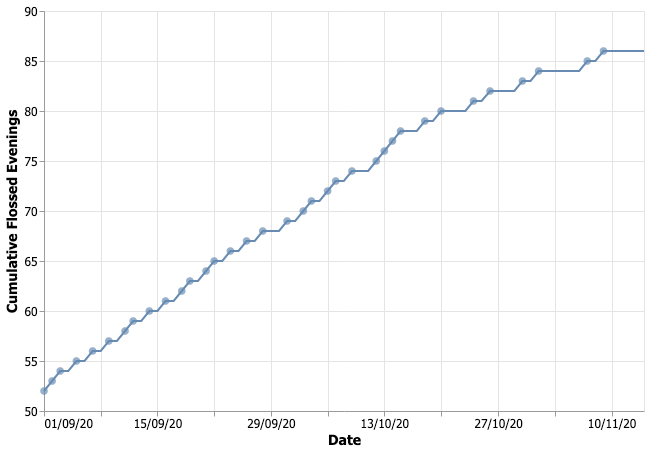
It’s pretty obvious that my flossing rate has changed around half of October. My goal was to reach this conclusion more formally, using PyMC3. It’s not the most exciting analysis, and the solution is borrowed from a StackOverflow answer 1, but it makes for good writing exercise (and I now also have a Beeminder goal that forces me to write things here).
First, I needed some data processing to obtain my flossing rate by using pandas.date_range and a join. Once the data is ready, the PyMC3 code for the model looked like this:
df = flossing_data

with pm.Model() as model:
    # Priors

    sigma = pm.HalfCauchy('sigma', beta=10, testval=1.)

    switch_lower = df["index"].min()
    switch_upper = df["index"].max()
    switchpoint = pm.DiscreteUniform('switchpoint', lower=switch_lower, upper=switch_upper)

    ## Priors for the intercept are informative

    intercept_u1 = pm.Uniform('Intercept_u1', lower=0.1, upper=.75)
    intercept_u2 = pm.Uniform('Intercept_u2', lower=0.1, upper=.75)

    # Model

    x = df["index"].values
    y = df["value"].values

    intercept = pm.math.switch(switchpoint > x, intercept_u1, intercept_u2)

    # Likelihood

    likelihood = pm.Normal("value", mu=intercept, sd=sigma, observed=y)

with model:
    step1 = pm.NUTS([intercept_u1, intercept_u2,])
    step2 = pm.Metropolis([switchpoint])

    trace = pm.sample(1000, step=[step1, step2], start=start, progressbar=True, cores=2, tune=2000)
The parameter of interest was “switchpoint” and here’s how the posterior samples for this parameter looked, alongside the data itself:
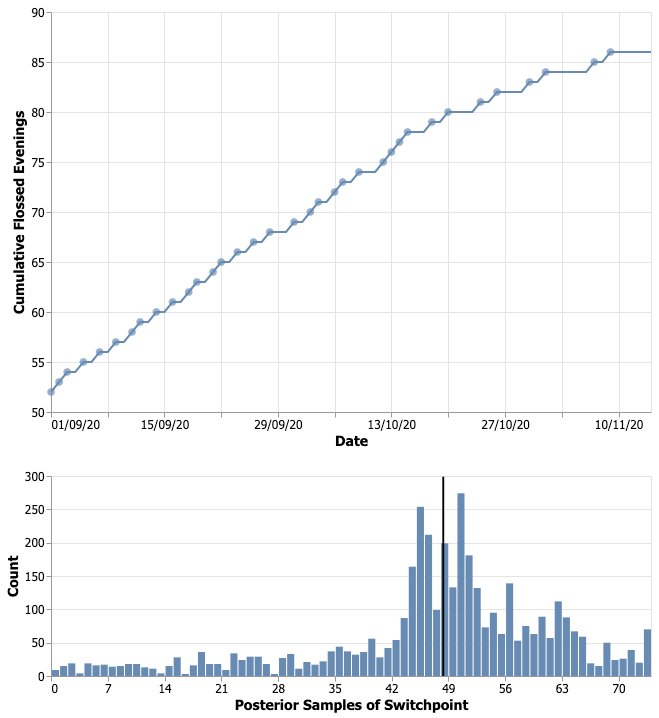
The model hedged its bet around the 48th day. Remarkably, the 94% probability range covers 17th to 74th day. This is largely due to the uninformative prior on the switchpoint parameter. We could have done better by specifying a prior that are a bit more informative and reduce the weight on the earlier and the later days.
Next to the parameter of interest, the “Intercept_u1” and “Intercept_u2” parameters could be interpreted as the daily rates of flossing and before and after the switchpoint, respectively:
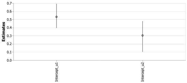
So the rate with which I flossed seemed to have decreased. In fact, we can test the hypothesis directly using the posterior samples:
posterior_intercepts = pm_data.posterior[["Intercept_u1", "Intercept_u2"]].to_dataframe()
h_u1_gt_u2 = posterior_intercepts["Intercept_u1"] > posterior_intercepts["Intercept_u2"]

h_u1_gt_u2.mean()
# > 0.93925
Looking at the data, the probability that I flossed more while using Beeminder than in the period I haven’t used it is 94%.
This is a neat, albeit a trivial, example. I did learn a few elementary details about Bayesian estimation using PyMC3 in the process and it served me as a writing exercise.