Put blandly, a Dirichlet process is a stochastic process whose realisations are probability distributions. It has two parameters: a base distribution and a scaling parameter.

In Bayesian statistics, the Dirichlet Process is useful when modeling, for instance, a random variable which has a mixture of normal distributions and we aren’t sure how many components are involved. As such, it is a nonparametric Bayesian model.

I recently had a problem at work that I though could be solved by modeling it as a Dirichlet Process, but I didn’t feel confident enough and solved it using a few linear regression models. What’s a better excuse to practise some writing?

Let’s quickly visit the notation for a Dirichlet Process. A random variable $Y$ is a Dirichlet process:

where $N$ stands for normal distribution and $\alpha$ is the scaling parameter of the Dirichlet process. $\alpha$ has a natural interpretation: The lower the value, the less spread realisations of $Y$ will be around $N$. In the context of mixture distributions, $\alpha$ conveys information as to how many components there will be in the mixture.

Now let’s consider the following made up case: We’re asked to model the number of cars that enter the city of Utrecht per hour. The stakeholders involved are the city planners and they know that the average number of cars that enter the city can be modeled by using period of day. For instance, the average in the morning hours might be:

In the noon, however, the location of the normal distribution will shift to $\mu_{noon}$ ¹.

Let’s also suppose that they’re willing to reconsider their definitions for period of day, and would like to see what the data has to tell them. So part of our task is to summarise the evidence on this matter: The analysis should be flexible with respect to however many time periods there are.

We could approach this problem with the following model:

where we’d split the day into $K$ time periods, each time period would be modeled by a different normal distribution $N(\mu_i, 1 / {\tau_{i}\lambda_{i}})$ and each data point would belong to one of these with probability $w_i$.

Now, let’s build up the components of this model. Since we want to time periods to be similar to each other in terms of average number of cars, we’ll estimate $\mu_i$ by using an intercept only linear model,

We’ll use the Dirichlet process for modeling $w_i$s:

where

are the parameters for the Dirichlet process.

We can get this far by simply following the relevant PyMC3 documentation. When learning something like this, building up the conceptual understanding up to this basic point and playing with an example is a good method, I think. So let’s make sure we can actually make sense of model output based on what we understood so far.

Dummy example

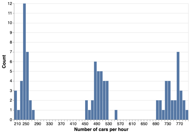
Let’s create some data with a structure that will make the job easy for this kind of model.

generator = np.random.default_rng()
size = 30

dat_count = np.vstack([
    generator.poisson(lam=750, size=(size, 1)), # morning
    generator.poisson(lam=500, size=(size, 1)), # noon
    generator.poisson(lam=250, size=(size, 1)), # evening
])

dat_period = np.vstack([
    np.asarray(["morning"] * size),
    np.asarray(["noon"] * size),
    np.asarray(["evening"] * size),
]).reshape(-1, 1)

dat = np.hstack([
    dat_count,
    dat_period
])

df_count = pd.DataFrame(dat, columns=["count", "period"], )
df_count["count"] = df_count["count"].astype(int)

This is a dataset with three, clearly distinct groups:

We can standardise the count column and we have our $y$:

count_mean = df_count["count"].mean()
count_sd = df_count["count"].std()
df_count["count_std"] = (df_count["count"] - count_mean) / count_sd

Following the tutorial, we can fit a Dirichlet Process model like so:

K = 30

def stick_breaking(beta):
    portion_remaining = tt.concatenate([[1], tt.extra_ops.cumprod(1 - beta)[:-1]])
    
    return beta * portion_remaining

with pm.Model() as m:
    alpha = pm.Gamma("alpha", 1, 1)
    beta = pm.Beta("beta", 1, alpha, shape=K) 
    w = pm.Deterministic("w", stick_breaking(beta))
    
    tau = pm.Gamma("tau", 1.0, 1.0, shape=K)
    lambda_ = pm.Gamma("lambda_", 10.0, 1.0, shape=K)
    mu = pm.Normal("mu", mu=0, tau=tau * lambda_, shape=K)
    
    obs = pm.NormalMixture(
        "obs", w, mu, tau=lambda_ * tau, observed=y["count_std"].values
    )
	
with m:
    trace = pm.sample(500, tune=500, chains=3, cores=3, init="advi", target_accept=.875) 	

I’ll jump over the model checks… since at this point I went into a rabbit hole that swallowed my hours. The rabbit I chased looked like this:

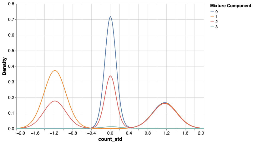
How is it possible that for instance component 2 is multimodel, while I specified it as a normal distribution? This is yet another way of observing what’s called label switching. This isn’t big of a concern if you’re after the marginal density. But is a bit of an issue if you’re after clustering your data points into these components.

It turns out, fitting Dirichlet Process mixtures is rather hard. And hard problems in Bayesian statistics are really frustrating when you’re not experienced with the model you’re working, because you may need to wait 30 minutes to get a result that you can’t even use.

There seem to be different ways of dealing with this issue, which I’d like to get back to soon.

Before that, however, I’ll turn to something else that I came to know while I was reading about this problem: variational inference. Sayam Kumar has talk on this topic titled “Demystifying Variational Inference which he advertises with the following questions “What will you do if MCMC is taking too long to sample? Also what if the dataset is huge? Is there any other cost-effective method for finding the posterior that can save us and potentially produce similar results?”

More on variational inference to come!